Journal of Fluid Flow, Heat and Mass Transfer (JFFHMT)
ISSN: 2368-6111

Volume 4 - Year 2017 - Pages 36-46
DOI: 10.11159/jffhmt.2017.005
Steady Streaming Motion in Entrance Region of Curved Tubes during Oscillatory Flow
Masaru Sumida
Kindai University, Faculty of Engineering
1 Takaya Umenobe, Higashi-Hiroshima, 739-2116, Japan
sumida@hiro.kindai.ac.jp
Abstract - An experimental investigation was carried out on the development of oscillatory laminar flow in curved tubes with a turn angle of 180° (i.e., U-shaped tubes) and curvature radius ratios Rc of 4 and 10. Experiments were conducted under Womersley numbers a of 18 to 30 and Dean numbers D of 150 and 300, giving b (=a2/D) above 0.655, for which the characteristics of the oscillatory flow in the fully developed region of the curved tubes are roughly divisible into two. The secondary flow induced in the cross section was visualized by a solid tracer method with a stroboscopic light and was recorded photographically at several stations upstream and downstream from the entrance of the curved tube. The development of the secondary flow and transitions between the straight-tube and curved-tube oscillatory flows were systematically investigated in detail. Two pairs of vortices, the so-called Lyne circulation, for high b values appear even at the entrance. The classification of the secondary-flow pattern observed for the fully developed region is applicable to the region developing downstream from the entrance. Accompanying the secondary-flow development, in the straight section immediately before the entrance, a steady streaming occurs in the symmetrical horizontal plane. Furthermore, the steady streaming forms an elliptical trajectory with an increase in a. Both the streamings generated in the oscillating boundary layer near the entrance show very complicated behaviors.
Keywords: Oscillatory flow, Steady streaming, Curved tube, Secondary flow, Entrance region, Womersley number.
© Copyright 2017 Authors - This is an Open Access article published under the Creative Commons Attribution License terms Creative Commons Attribution License terms. Unrestricted use, distribution, and reproduction in any medium are permitted, provided the original work is properly cited.
Date Received: 2017-06-07
Date Accepted: 2017-10-10
Date Published: 2017-12-01
Nomenclature
- a: radius of tube, a=d/2 (d: tube diameter)
- D: Dean number, D =Re Rc-1/2
- Q: Flow rate
- R: curvature radius of tube axis
- Rc: curvature radius ratio, Rc=R/a
- Re: Reynolds number, Re =2awm,o /n
- S: secondary flow velocity
- T: oscillation period, T = 2p/w(w : angular frequency)
- u, v, w: velocities in x, y and z directions, respectively
- wm: axial velocity averaged over cross section
- x, y, z: coordinate system, see Figure 3
- a: Womersley number, a = a(w/n)1/2
- b: characteristic parameter, b=a2/D
- Q: phase angle, Q = w t (t: time)
- n: kinematic viscosity of fluid
- r: density of fluid
- W: turn angle, see Figure 3
- Subscripts
- m, x: average values over cross section and x-axis, respectively
- ta, o: time-mean and amplitude values, respectively
1. Introduction
The purpose of this study is to investigate the flow field near the bend entrance of curved tubes during oscillatory flow. To this end, we perform a visualization experiment and velocity measurement on both the steady streaming and the secondary flow motion induced in the horizontal and vertical planes, respectively. We examine the flow characteristics in the entrance region including that of a straight tube connected to a curved tube.
The focus of the study on flows in curved tubes has proceeded from the practical standpoint of obtaining pressure and energy losses in the past to the elucidation of the mechanism of the flows. An interesting subject of discussion among researchers is secondary flow motion. A secondary flow is generated, owing to the action of the centrifugal force on the fluid, in the cross-sectional plane perpendicular to the tube axis. Many researchers of internal fluid dynamics have experimentally, theoretically and/or numerically investigated the secondary-flow problem [1]-[4].
In particular, great interest has been focused on unsteady flows since Lyne [5] and subsequently Zalosh and Nelson [6] analytically predicted two pairs of vortices for a fully developed oscillatory flow. The secondary flow observed by them is different from the familiar Dean vortices of a steady flow. A few experiments have been conducted to confirm Lyne’s prediction. Visualization studies were carried out by Lyne [5] and Munson [7] using a dye injection method and by Bertelsen [8] using an aluminum-powder tracer technique. Unfortunately, however, their experiments were limited to qualitative observations to demonstrate the existence of the new secondary flow predicted by Lyne [5] because of the limitations of the visualizing methods employed. Therefore, these studies have not led to a demonstration that the strength of the secondary-flow motion depends on both the oscillation frequency and the amplitude of the reciprocating velocity.
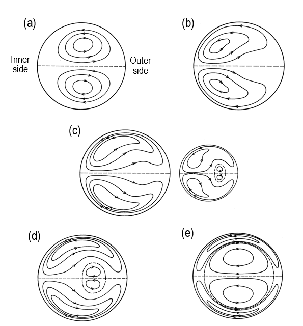
Considering the above situation, the author’s group [9], [10] developed a new method for visualizing the secondary motion for both steady and unsteady flows. This method is a type of multi-exposure solid-tracer method using a stroboscopic light. By this method, one can readily and simultaneously obtain not only the pattern but also the velocity information of the secondary-flow field. First, this method was applied to a fully developed oscillatory flow in a circular curved tube with a curvature radius ratio Rc of 7.6 [10], where Rc=R/a is the ratio of the curvature radius of the tube axis R to the radius of the tube a. The important results obtained were that the oscillatory flow is mainly governed by the Womersley number a and the Dean number D, and that the pattern of the secondary flow formed in the cross section can be classified into five patterns including Lyne circulation, as shown in Figure 1. Here, the Womersley number is a nondimensional frequency parameter and is defined as a=a(w/n)1/2 with w being the angular frequency of oscillation and n the kinematic viscosity of the fluid. The Dean number is expressed as D=ReRc-1/2, where Re=2awm,o/n is the Reynolds number with wm,o being the amplitude of the instantaneous axial velocity wm averaged over the cross section. The Womersley number can be physically interpreted as the square root of the ratio of the unsteady inertia force to the viscous force, while the Dean number is the ratio of the square root of the product of the inertia and centrifugal forces to the viscous force. The classification can also be quantitatively determined according to the magnitudes of a and D. However, the above study and its findings were concerned with the secondary flow for a fully developed region. Hence, our interest further extends to the secondary flow that develops in the entrance region of circular curved tubes.
Note that the fluid near the bend entrance reciprocates in the direction of the axis between the curved and straight sections in one cycle. Therefore, during half of the cycle, the fluid there is subjected to a centrifugal force, which causes a secondary flow in the curved section. Subsequently, the fluid exits the curve and enters the straight section during the other half cycle. Hence, the secondary motion is alternately driven and extinguished along the tube axis. In addition, the strength of the secondary-flow motion changes greatly in the axial direction.
Thus, the secondary flow in the entrance region is predicted to interfere with axial flow development, changing it in a complicated manner. Few studies have been reported on the oscillatory entrance flow in a curved tube. Bertelsen and Thorsen [11] and Naruse et al. [12] considered axial flow development. In the study of Bertelsen and Thorsen [11], profiles of the axial and outward velocities in a symmetrical horizontal plane were merely examined. Thus, the behavior of the secondary flow induced in a cross section near the entrance of curved tubes, at least to the author’s knowledge, has not been investigated in detail.
This paper is concerned with the development of the secondary flow motion generated in the vicinity of a curved tube with a straight section connected to each end of the curved tube. In particular, we examine a high-Womersley-number flow problem, in which the secondary flow shows a peculiar pattern, i.e., Lyne circulation. Subsequently, we discuss the effects of the governing parameters a, D and Rc on the development of the secondary flow. Moreover, we describe the relationship between the secondary flow development and the additional steady streaming essentially formed in the horizontal plane.
This type of unsteady flow problem has arisen in the field of physiology because of the strong interest in the flow in the cardiovascular system. To apply the results of the oscillatory flow in curved tubes to such flows, the flow near the entrance is more important than that in the fully developed region. Thus, this study is expected to contribute to the field of physiology.
2. Experimental Apparatus and Procedures
2. 1. Experimental Apparatus
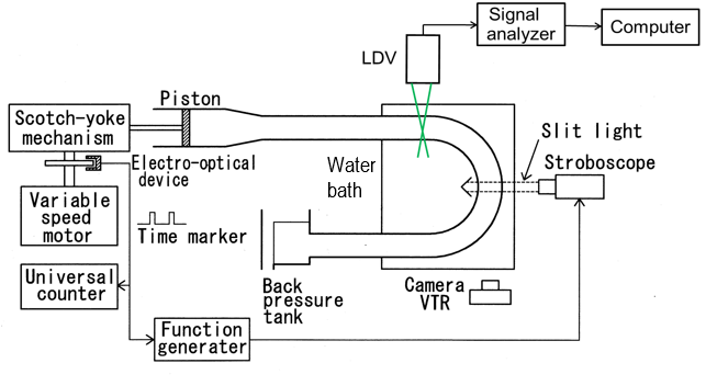
The experimental apparatus employed in the present study is shown schematically in Figure 2. The apparatus consists of an oscillatory flow generator, a test tube, and visualizing and measuring devices. An oscillating water flow was generated by a piston pump installed in a scotch yoke mechanism. Then, the desired volume-cycled flow rate Q was obtained by the selection and adjustment of the diameter (6, 10 and 15 mm) and stroke (0-60 mm) of the piston, and by adjusting the rotational frequency of a variable speed motor. The instantaneous flow rate Q (t) is given by

where Q(=wt) is the phase angle, w the angular frequency, t time and the suffix o the amplitude. The amplitude of the volumetric flow rate Qo is related to wm,o by wm,o= Qo/(pa2).
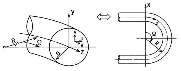
Figure 3 shows the coordinate system and the configuration of the test curved tube. Two curved tubes with a turn angle of 180°, namely, U-shaped tubes (U tubes), were employed in the present study. They were made of transparent glass. The internal diameters were d (=2a) =14.3 and 17.6 mm, and the curvature radii of the tube axis were R=72 and 35 mm, respectively. The thicknesses of the tubes were 1.8 and 1.2 mm, respectively. These dimensions give curvature radius ratios Rc (=R/a) of 10 and 4, respectively. The straight sections of the U tubes had a length of about 70d. The test tube was placed in a transparent water bath to reduce optical distortion when carrying out photography and to keep the water temperature at 20°C. The setting procedures are illustrated in Figures 5 and 6, as described later.
2. 2. Flow Visualization and Velocity Measurement
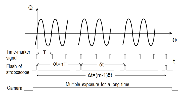
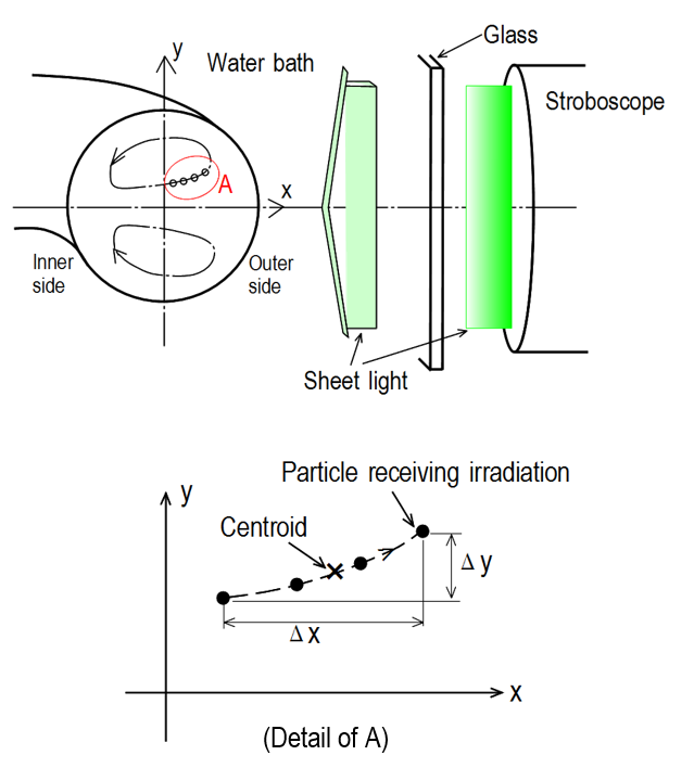
Visualization experiments were conducted for both the secondary stream occurring in the cross section and the steady streaming generated in the horizontal plane including the tube axis. The fluid flows were rendered visible by a solid tracer method using a stroboscopic light. The procedures used for irradiation with the stroboscope and recording with a camera are presented in Figure 4. Furthermore, Figures 5 and 6 concretely show the positional relationships between the measured fluid layers of the secondary stream and steady streaming and the stroboscope and the camera, respectively. This technique was developed by Sumida et al. [9] and Sudo et al. [10], as indicated in the introduction. When the Womersley number is high, the fluid in the tube goes and comes back almost in the same phase as the reciprocating piston pump, and the axial flow velocity becomes approximately uniform except near the tube wall. Consequently, the fluid particles in an irradiated plane at a given phase Q return to positions close to the initial ones after one cycle, i.e., Q+2p. The present method is suitable for the measurement of such a reciprocating flow in which the distance between the positions of a fluid particle at the beginning and end of a cycle is extremely small.
The tracers used were spherical white nylon particles with a diameter of about 90 mm and a specific gravity of 1.01-1.02, which were chosen in consideration of their responsiveness to flow variations.
They were introduced into the water at a weight ratio of 1 to 10-4. The fluid layer to be rendered visible was irradiated with the parallel sheet light from a condenser stroboscope.
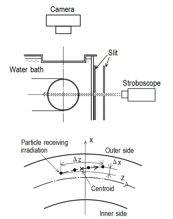
Firstly, measurements of the secondary stream in the cross section were performed at four streamwise stations between z=-d in the upstream tube and W=30° in the curved tube. Sheet light with a thickness of 2-3 mm was applied to the cross section (x-y plane) perpendicular to the tube axis, as shown in Figure 5. The fluid layer was irradiated once, at the phase of Q=0°, every 1 to 4 oscillation cycles, as demonstrated in Figure 4. Furthermore, the irradiation was repeated 4 to 20 times and the paths of the tracer particles during this period were photographed with a multiple exposure for a long time. In this case, the flash interval dt of the stroboscope was dt=nT, where T is the oscillation period 2p/w and n takes values of 1-4. Moreover, this visualization technique was also applied to the steady streaming in the horizontal (x-z) plane including the tube axis, as shown in Figure 6. In this case, the thickness of the sheet light was about 1 mm. The velocity information obtained from the steady streaming generated in the symmetrical plane should be useful in understanding the development of the secondary stream in the cross section.
In these experiments, Lagrangian displacements of the fluid particles for several oscillation cycles were obtained photographically. Needless to say, their displacements per a cycle are very small since the secondary flow velocity S is at most about 1% of the axial flow velocity w, as discussed later in section 3.3. Consequently, we can consider that the obtained Lagrangian velocity is Eulerian at its corresponding position, i.e., the centroid of a sequence of trajectory points. Thus, the velocity calculated in this manner is time-averaged over one cycle. Also, it denotes the magnitudes of the secondary stream and the steady streaming occurring in the horizontal plane. Although the secondary stream in the cross section is also a steady streaming, we refer to it as the secondary stream to avoid confusion.
Concretely, these fluid velocities were obtained from the photographs as follows. The displacements of the tracer particles ( Dx, Dy) and (Dx, Dz) in the vertical and horizontal planes, respectively, were determined using a personal computer. Here,Dx, Dy and Dz are the components of the vectors in the x, y and z directions, respectively (see Figures 5 and 6). Then the corresponding time-averaged velocities uta, vta and wta at the centroid of the path line elements were calculated easily from D x/Dt, Dy/Dt and Dz/Dt, respectively. Here, the suffix ta indicates time-averaged values and Dt is the time required for the particle displacement, i.e., Dt=(m-1)dt with m being the number of irradiations.
The optical distortions due to the tube curvature were reduced by placing the test tube in a water bath as described in section 2.1. Nevertheless, the distortions when taking a photograph still remained as high as 3.1 and 2.6% near the tube wall for the secondary stream and the steady streaming, respectively. The points were corrected from the velocity vectors determined from the photographs. However, there was a 1.6% error in the reading of the positions of irradiated particles by the computer. This led to errors in the velocities, which were estimated to be 4 and 3% of the local secondary stream and axial velocities, respectively. Consequently, the total measurement error was estimated to be less than 7% except near the tube wall. In addition, the error for the secondary stream was large compared with that for the steady streaming, particularly in the straight section far from the bend entrance.
2. 3. LDV Measurement of Axial Flow Velocity
For the axial flow, the velocity was also measured using a laser Doppler velocimeter (LDV; Kanomax Co. Ltd., System 8832), in which the laser source was a 3 W argon ion laser operated in the backscattering mode. The system was mounted on a traversing device controlled by a personal computer. It was aligned at a prescribed position with accuracy within 0.05 mm in the direction of the x-axis. The test tube was placed in a water bath to reduce the effect of the refraction of the conduit wall on the laser beam optics, as shown in Figures 1 and 6. This mitigates the curvature effect that leads to errors in the cross angle of the laser beam and in the positioning of the measuring volume. Nevertheless, total measurement errors of 4% remained in the local velocity except near the tube wall, whereas they were estimated to be 6% for the velocity in the boundary layer. The details of the measurement method and the error are given in an earlier work [2].
3. Results and Discussion
The secondary flow induced in the cross section of the fully developed region can be classified into five patterns, as stated in the introduction. According to the findings of Sudo et al. [10], for low Womersley numbers, the time- and cross-sectional-averaged velocity Sta,m of the secondary flow increases in proportion to the Dean number. On the other hand, when the Womersley number exceeds a specific value, the secondary flow velocity Sta,m decreases sharply and then changes in proportion to D2/a2.5.
In particular, at high values of the characteristic parameterb(=a2/D), i.e., b> 0.655, unsteady inertia effects predominate in the core region of the curved tube, while viscous effects are restricted to a thin layer adjacent to the tube wall. In the cross section, an additional pair of vortices rotating in the opposite direction to the primary vortices is generated in the core region. Therefore, two pairs of vortices are formed in the cross section of the curved tube. This secondary flow pattern is well known as Lyne circulation [5].
In the following section, we consider the oscillatory flow for a b value considerably higher than 0.655, at which the secondary flow pattern is divided roughly into two. Furthermore, we discuss the effects of the Womersley number on the Lyne-type secondary flow near the entrance of the curved tube. Also, we reveal the features of the oscillatory entrance flow.
3. 1. Development of Secondary Stream in the Cross Section
For high bvalues, the unsteady inertia force exerted on the fluid has a significant effect as stated above. Consequently, the fluid develops reciprocating motion throughout the tube, in which the axial velocity shows an annular profile, taking a maximum at the edge of the oscillating boundary layer in the neighborhood of the tube wall.
Figure 7 shows a typical example of the trajectory of the fluid particles in the horizontal plane of the curved tube, together with a schematic diagram showing the imaged section. The photograph was taken by a multi-exposure method involving two exposures using a continuous sheet light during a half cycle to visualize the fluid motion. From the photograph, the fluid particles were observed to exhibit reciprocating motion in the W and zdirections along the tube axis at the fundamental oscillation frequency. They also slightly shift in the centripetal direction simultaneously. The former indicates that the distance moved by a fluid particle during one cycle is equivalent to 2wo/w, where wo is the fundamental oscillating component of the axial velocity w. The latter denotes the time-averaged velocity uta, obtained as Dx/Dt, in the horizontal (x-z) plane. Such a time-averaged flow is called a steady streaming.
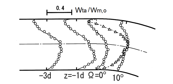
The profiles of the axial-velocity amplitude wo are shown in Figure 8, in which wo was evaluated from the lengths of pathlines along the tube axis and also obtained using LDV. The LDV measurements were performed at stations selected with reference to the visualization results. In Figure 8, the solid line at the station of W= 70 to 90° indicates the results of Sudo et al. [10] for a fully developed region, which were obtained by numerical analysis. Furthermore, the triangles show the experimental data obtained by Bertelsen and Thorsen [11] using LDV at W=1.03° for Rc=4 [b=1.54 (a=21.8, D=308)]. For oscillatory flow in tubes [13], when the Womersley number becomes large, the viscous effects become restricted to the neighborhood of the tube wall and the inertia effects increase relatively in the central region of the tube. The fluid in the central region cannot strictly follow the variation in the axial pressure gradient compared to the fluid near the wall. This causes the axial velocity to have an annular profile that takes the form of a crest near the wall. In the curved tube with Rc=4 shown in Figure 8, the axial-velocity amplitude wo increases near the inner wall along the direction of W from the straight section close to the entrance. This finding has also been observed in a curved tube with Rc=10. A change in the wo profile along the tube axis has been reported by Bertelsen and Thorsen [11]. On the other hand, the displacement of the pathlines in the negative x direction exemplifies the existence of a steady secondary flow toward the inner wall from the outer wall in the horizontal (symmetrical) plane at the same time.
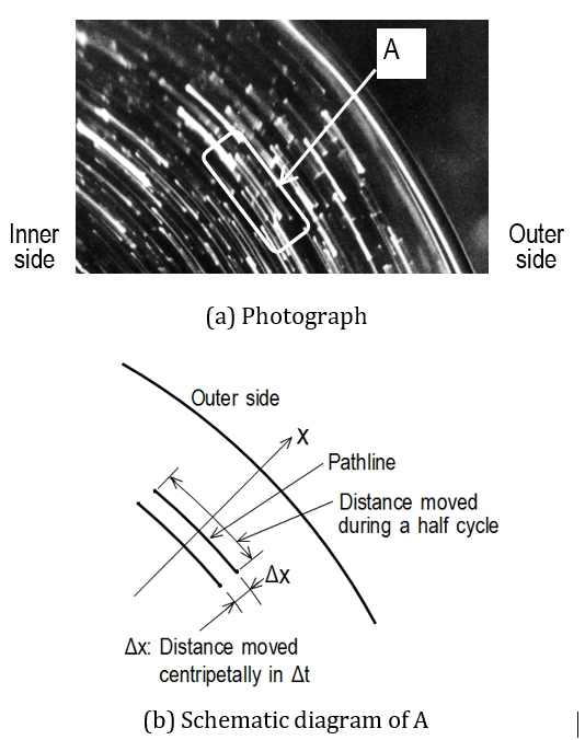
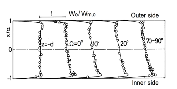
Figure 9 shows the development of the secondary flow generated in the cross section perpendicular to the tube axis. The motion readily obtained from the photographs indicates the time-averaged secondary stream because it is a steady streaming. The velocity vectors in Figure 9 are drawn on the basis of several photographs taken under the same flow conditions. For the flow at b=1.08, the secondary stream in the fully developed region shows almost typical Lyne circulation. In the photographs shown in Figure 9, the oscillating component of the secondary flow is not observed, while the sequence of the trajectory points of nondiffusive tracer particles denotes only the time-averaged velocity of the secondary flow. It is observed that the fluid particles in the cross section slightly shift their positions in each reciprocating axial motion. Furthermore, the secondary stream with two pairs of vortices still appears at the entrance plane of W=0°. Nevertheless, the secondary stream with vortices begins to vanish near the outer wall in the straight tube and the secondary motion at the plane of z=-1d barely exists near the inner-wall side of the x-axis.
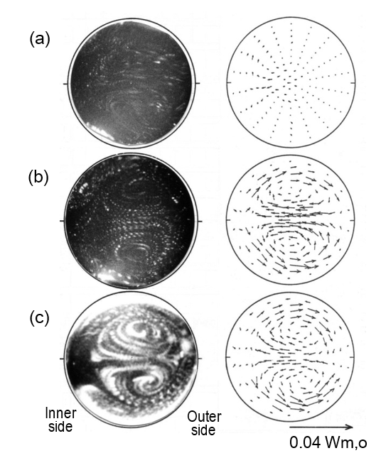
(a) z= -1d. (b) W=0°. (c) W=20°.
3. 2. Steady Streaming in Horizontal Plane
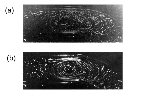
The secondary stream mentioned above is well known as a steady streaming [14], the existence of which was revealed by observation during several oscillation cycles. Similarly, the steady streaming generated in the horizontal plane including the tube axis can be observed by the present flow visualization technique as described in section 2. Examples of results obtained photographically are provided in Figure 10 for b=1.08 (a=18) and b=3.0 (a=30). A vector diagram is included for the case of b=1.08. For b=1.08 in Figure 10(a), the steady streaming has larger velocities at the edge of the oscillating boundary layer. Moreover, the steady streaming flows clockwise and its center lies in the straight section upward from the bend entrance, that is, it is in the W and negative z directions in the outer and inner regions of the horizontal plane, respectively. This results from the fact that in the vicinity of the curved-tube entrance, the amplitude of the axial velocity wo at the edge of the oscillating boundary layer changes in the W direction as observed in Figure 8. To put it more concretely, for a change in the wo profile, a velocity component normal to the oscillating boundary layer is required as an inevitable consequence of the relation of mass conservation. Therefore, the fluids near the outer and inner walls flow out of and into the oscillating boundary layer, respectively. Thus, the steady streaming becomes strong in the region where wo at the edge of the oscillating boundary layer changes abruptly in the z or W direction.
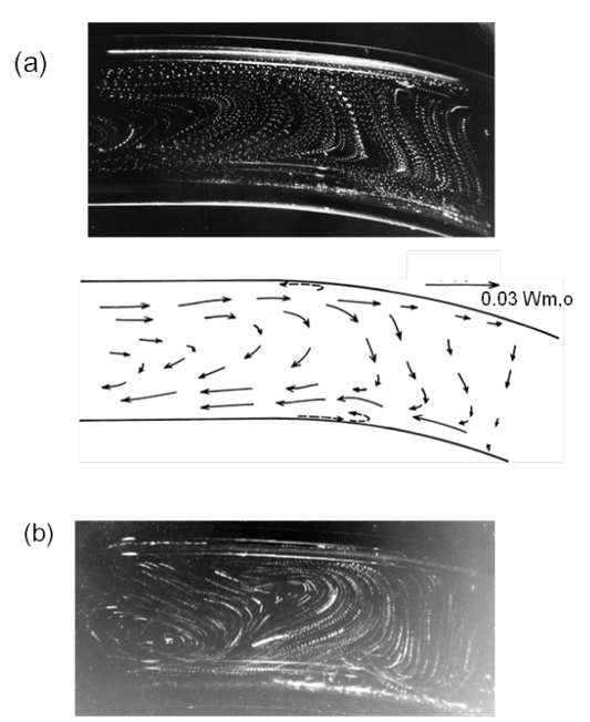
(a) b=1.08 (a=18), dt=T. (b)b=3.0 (a=30), dt=2T.
On the other hand, in the interior of the oscillating boundary layer near the entrance, another incidental streamings are also induced, as illustrated by broken lines in the vector diagram shown in Figure 10(a). The additional streamings result from the fact that the centrifugal force acting on the fluid there, where the amplitude of the axial velocity is locally large, is directed toward the outer wall regardless of the direction of the primary flow. The streamings circulate within the oscillating boundary layer adjacent to the tube wall. From these findings, the steady streamings generated in the horizontal and symmetrical planes show a double structure. The steady streaming in the core region is observed in the opposite direction to the recirculating flow for low a values, i.e., b<0.655, as in Figure 11 [15]. In Figure 11, the data indicated by the triangle are the velocity distributions estimates of Naruse's et al. [12]. Such a steady streaming phenomenon depending on a and/or b is a very interesting effect of a nonlinear action for the oscillatory entrance flow in curved tubes.
3. 3. Strengths of Secondary Stream and Steady Streaming
Comparing the secondary stream in the cross section with the steady streaming in the horizontal plane in Figures 9 and 10, respectively, we can clearly observe the transition between the straight- and curved-tube oscillatory flows. The flow mechanism of the secondary stream and the steady streaming is schematically illustrated in Figure 12. The steady streaming in the inner part of the horizontal plane immediately upstream from the entrance is toward the inner-wall side. The vortex motion of the secondary stream begins to collapse in the outer part of the cross section. In the curved section, on the other hand, the steady streaming in the horizontal plane changes its direction to the centripetal direction with an increase in W.
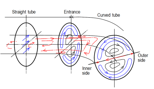 Figure 12. Schematic
diagram showing the relation between the secondary stream and the steady
streaming near the bend entrance. Blue and black lines show the secondary
stream in the cross section, and red lines denote the steady streaming in the
horizontal (symmetrical) plane.
Figure 12. Schematic
diagram showing the relation between the secondary stream and the steady
streaming near the bend entrance. Blue and black lines show the secondary
stream in the cross section, and red lines denote the steady streaming in the
horizontal (symmetrical) plane.
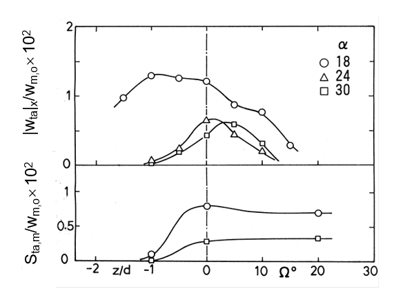
To estimate the strengths of the secondary stream and the steady streaming, we introduce the quantities |wta|x and Sta,m, respectively. Here, |wta|x is the average of |wta| over the x-axis, |wta| being the absolute value of the time-averaged axial velocity wta of the steady streaming. Sta,m denotes the cross-sectional average value of Sta, which is the secondary stream velocity described by Sta= (uta2 + vta2)1/2. Figure 13 shows the changes in |wta|x and Sta,m along the tube axis. For a=18 (D=300), the strength Sta,m of the secondary stream is slightly larger at the bend entrance but does not reach 1% of wm,o, while the change in Sta,m in the curved section of the tube is small. On the other hand, |wta| x, denoting the strength of the steady streaming in the horizontal plane, is largest in the section of z»-1d, at which the center of the streaming is located. However, it decreases further away from the center. Furthermore, both the secondary stream and the steady streaming weaken with an increase in a, since the unsteady inertia force increases so that the change in the wo profile in the W direction decreases. For higher b ranging from 10.4 to 32.0, Bertelsen [8] measured the time-averaged secondary-stream velocity uta on the x-axis in a fully developed region with Rc=9.26. Regarding the average of |uta| over the x-axis estimated from his data, |uta|x/wm,o gives a value of (0.3-0.7)´10-3. The value is approximately one-tenth of that in the present data for b=1.08-3, appearing to be of an inverse ratio of b.
The results for a curved tube with a strong curvature (Rc=4) are given in Figures 14-16. When the tube curvature becomes strong, the steady streaming in the horizontal plane forms a planar elliptical shape circulating clockwise, as shown in Figure 14. In addition, the center of the streaming is located at a point closer to the bend entrance, but the position does not significantly change with a and D. Following this, the Lyne-type secondary flow with two pairs of vortices begins to be distorted in the outer and subsequently inner parts of the cross section at the entrance plane (W=0°). Photographs showing this phenomenon are provided in Figure 15. Consequently, the secondary motion in the section of z»-1d beyond the center of the steady streaming in the horizontal plane changes into a flow that faces the outer wall in the central part of the cross section.
(a) b=1.08 (a=18), dt=T. (b) b=3.0 (a=30), dt=2T.
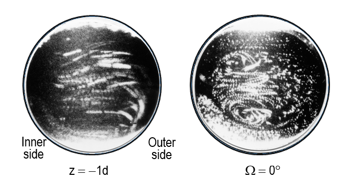
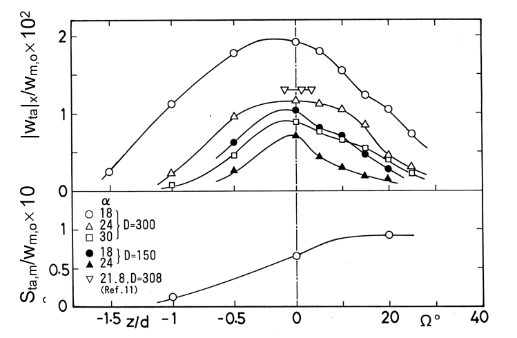
Figure 16 shows the values of Sta,m and |wta|x for the strongly curved tube. The strength Sta,m of the secondary stream in the section of the curved tube does not differ significantly from the case of Rc=10 for the same value of D. However, the ratio of Sta,m to wm,o, Sta,m /wm,o, changes proportionally to Rc-1/2 [10]. On the other hand, the strength |wta|x of the steady streaming is highest at the section closer to the entrance at which the center of the steady streaming is located. It is about two times as large as Sta,m for the secondary stream. According to the experiments in reference [11], |uta|x/wm,o is estimated to be 0.32´10-2 at the station of z=-0.0955d, for a=21.8 and D=308, in the curved tube with Rc=4. This supports to our results. As the Dean number decreases, |wta|x decreases.
4. Conclusions
Flow visualization experiments were performed for the oscillatory entrance flow in curved tubes. The important findings drawn from the present results for a high characteristic parameter, b>0.655, are as follows:
- The classification of the secondary-flow pattern for the fully developed oscillatory flow is applicable to the flow developing downstream from the bend entrance. Two pairs of vortices, the so-called Lyne circulation, appear even at the bend entrance.
- The strength of the secondary stream developing in the curved section does not change markedly and is roughly equal to that in the fully developed region.
- For Rc=10, the secondary stream in the straight section decays near the outer and subsequently inner walls. For Rc=4, i.e., a strong curvature, the secondary motion in the plane of z»-1d shifts from inward to outward in the central part of the cross section.
- Accompanying such secondary-stream transitions, in the horizontal plane, a steady streaming is generated with a double structure. Furthermore, the trajectory of the fluid streaming drifts and forms an elliptical region with an increase in a, with the strength at the bend entrance about two times as large as that of the secondary stream.
References
[1] S. A. Berger, L. Talbot and L. –S. Yao, “Flow in curved pipes,” Annual Review of Fluid Mechanics, vol. 15, pp. 461-512. 1983. View Article
[2] M. Sumida, “Pulsatile entrance flow in curved pipes: effect of various parameters,” Experiments in Fluids, vol. 43, pp. 949-958, 2007. View Article
[3] B. Timité, C. Castelain and H. Peerhossaini, “Pulsatile viscous flow in a curved pipe: effects of pulsation on the development of secondary flow,” International Journal of Heat and Fluid Flow, vol. 31, pp. 879-896, 2010. View Article
[4] M. Jarrahi, C. Castelain and H. Peerhossaini, “Secondary flow patterns and mixing in laminar pulsating flow through a curved pipe,” Experiments in Fluids, vol. 50, pp. 1539-1558, 2011. View Article
[5] W. H. Lyne, “Unsteady viscous flow in a curved pipe,” Journal of Fluid Mechanics, vol. 45, no. 1, pp. 13-31, 1970. View Article
[6] R. G. Zalosh and W. G. Nelson, “Pulsating flow in a curved tube,” Journal of Fluid Mechanics, vol. 59, pp. 693-705, 1973. View Article
[7] B. R. Munson, “Experimental results for oscillating flow in a curved pipe,” Physics of Fluids, vol. 18, no. 12, pp. 1607-1609, 1975. View Article
[8] A. F. Bertelsen, “An experimental investigation of low Reynolds number secondary streaming effects associated with an oscillating viscous flow in a curved pipe,” Journal of Fluid Mechanics, vol. 70, pp. 519-527, 1975. View Article
[9] M. Sumida, K. Sudo and H. Wada, “Pulsating flow in a curved pipe: secondary flow,” JSME International Journal, Ser II, vol. 32, no. 4, pp. 523-531, 1989. View Article
[10] K. Sudo, M. Sumida and R. Yamane, “Secondary motion of fully developed oscillatory flow in a curved pipe,” Journal of Fluid Mechanics, vol. 237, pp. 189-208, 1992. View Article
[11] A. F. Bertelsen and L. K. Thorsen, “An experimental investigation of oscillatory flow in pipe bends,” Journal of Fluid Mechanics, vol. 118, pp. 269-284, 1982. View Article
[12] T. Naruse, Y. Nishina, H. Kugenuma and K. Tanishita, “Developing oscillatory flow in a strongly curved tube,” Transactions of Japan Society of Mechanical Engineers, vol. 56B, no. 529, pp. 2562-2569 (in Japanese), 1990.
[13] S. Uchida, “The pulsating viscous flow superposed on the steady laminar motion of incompressible fluid in a circular pipe,” Zeitshrift für Angewandte Mathematik und Physik, vol. 7, pp. 403-422, 1956. View Article
[14] D. P. Telionis, Unsteady Viscous Flows. New York: Springer, p. 154, 1981. View Book
[15] M. Sumida and K. Sudo, “Oscillatory flow in curved pipes, 4th report: velocity distribution in entrance region,” Transactions of Japan Society of Mechanical Engineers, vol. 60B, no. 569, pp. 63-70 (in Japanese), 1994.