Journal of Fluid Flow, Heat and Mass Transfer (JFFHMT)
ISSN: 2368-6111

Volume 3 - Year 2016 - Pages 86-91
DOI: 10.11159/jffhmt.2016.010
Flow around Nuclear rod bundles' simulations based on RANS and LES method respectively
Daqiang Yan, Jinghao Li
State Nuclear Power Software Development Center (SNPSDC)
National Energy Key Laboratory of Nuclear Power Software
South Park, Beijing Future Science & Technology City, Changping District, Beijing, China
yandaqiang@snptc.com.cn; lijinghao@snptc.com.cn
Abstract - The flow across the rod bundles in reactor pressure vessel is an essential design consideration of nuclear power plants. Experiments and CFD simulations are both effective methods for the rod bundles design and flow mixing analysis. CFD methods have the advantage of timesaving and cheaper, while experiment data is more reliable. Different turbulence models can be chosen in CFD simulation and the results are sensitive to the choice. So two kinds of turbulence model were investigated in this paper to evaluate their applicabilities in rod bundles CFD simulation. They are RANS and LES. The results were compared to experiment data, and the experiment is the flow in 3x3 rod bundles. The comparison between the CFD simulation and experiment data was shown in this paper for validation. The results showed that although there were some difference between the simulation and experiment, RANS and LES are both effective methods in nuclear engineering for simulating flow around rod bundles of fuel assembles. LES simulation can predict the velocity's peak value better and can be used for rod bundles design in nuclear design and research.
Keywords: Reactor, rod bundles, CFD, LES,RANS.
© Copyright 2016 Authors - This is an Open Access article published under the Creative Commons Attribution License terms Creative Commons Attribution License terms. Unrestricted use, distribution, and reproduction in any medium are permitted, provided the original work is properly cited.
Date Received: 2015-10-24
Date Accepted: 2016-10-11
Date Published: 2016-11-01
Nomenclature
- D: rod diameter, m
- Dh: hydraulic diameter of interior sub-channels,m
- G: gravity, acceleration, m/s2
- P: pressure, Pa
- Re: Reynolds number, ρ VDh/μ
- u: velocity vector, m/s
- w: axial velocity, m/s
- W: mean velocity in axial direction, m/s
- VD: Dimensionless axial velocity
- T: time, s
- X: horizontal coordinate, mm
- Y: vertical coordinate, mm
- Z: axial coordinate, mm
Greek letter
- ρ: density, kg/m3
- μ: dynamic viscosity, Pa s
1. Introduction
High performance of rod bundles' heat exchange is important to Pressurized Water Reactors' fuel assemble design [1]. CFD simulation is required to simulate the flow structure in order to understand and analysis the detail of the turbulence, mixing flow, velocity profile around rod bundles, as previously shown [2][3][7].
Although CFD has been used as a tool for analysis of reactor systems for more than 35 years [5], the spread use of CFD for designing a reactor is still limited. Whether the results of CFD simulation are accurate, it is still always in doubt. One reason is that CFD results are sensitively influenced by CFD users' experiences or choices. So more and more validation works have been done by many researchers [6][7][8]. The most reliable validation is comparing simulation results with analytic solutions in theory or experiment data.
In this paper, a 3x3 rod bundle experiment [9] was used to validate the simulation results. The objective of this paper was to evaluate the turbulence model choice in simulating the flow field around rod bundles of fuel assemble in reactors, and with the aid of experiment validation to find a proper turbulence model for engineering and research.
2. Introduction of experiment and simulation methods
2. 1. Experiment introduction
The 3x3 rod bundle experiment simulated in this paper is the facility installed in Shanghai Jiao Tong University. The facility full of water is used to validate the nuclear lumped methods codes for Pressurized Water Reactors. There are measuring window and Laser Doppler Velocimetry (LDV) system to measure the detail of water flow field at 1 atm. So the experiment data can also be used to validate CFD methods. The test section is shown in Figure 1 [9].
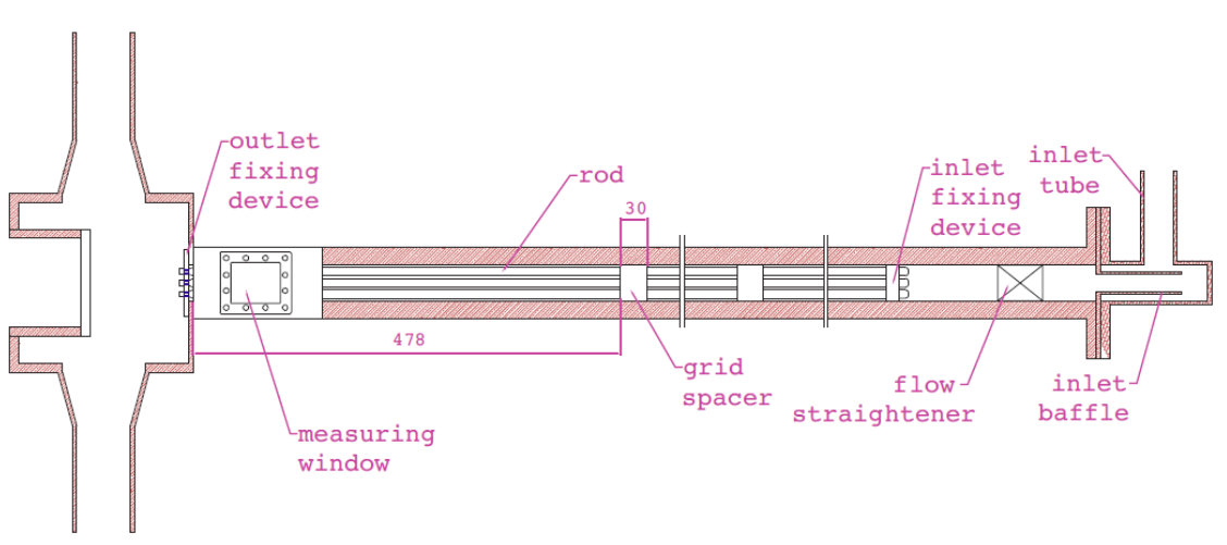
The bundles' length is 1.5m, their diameter is 9.5mm and the distance between bundles is 3mm. There are three grid spacers along bundles in every 0.48m. The bundles were fixed by the grid spacers. Another function of the spacers is enhancing the flow mixing among bundles, so that the bundles in a real reactor will have good performance for heat exchange. So there are highly mixing and remarkable turbulence flow in the experiment flow field.
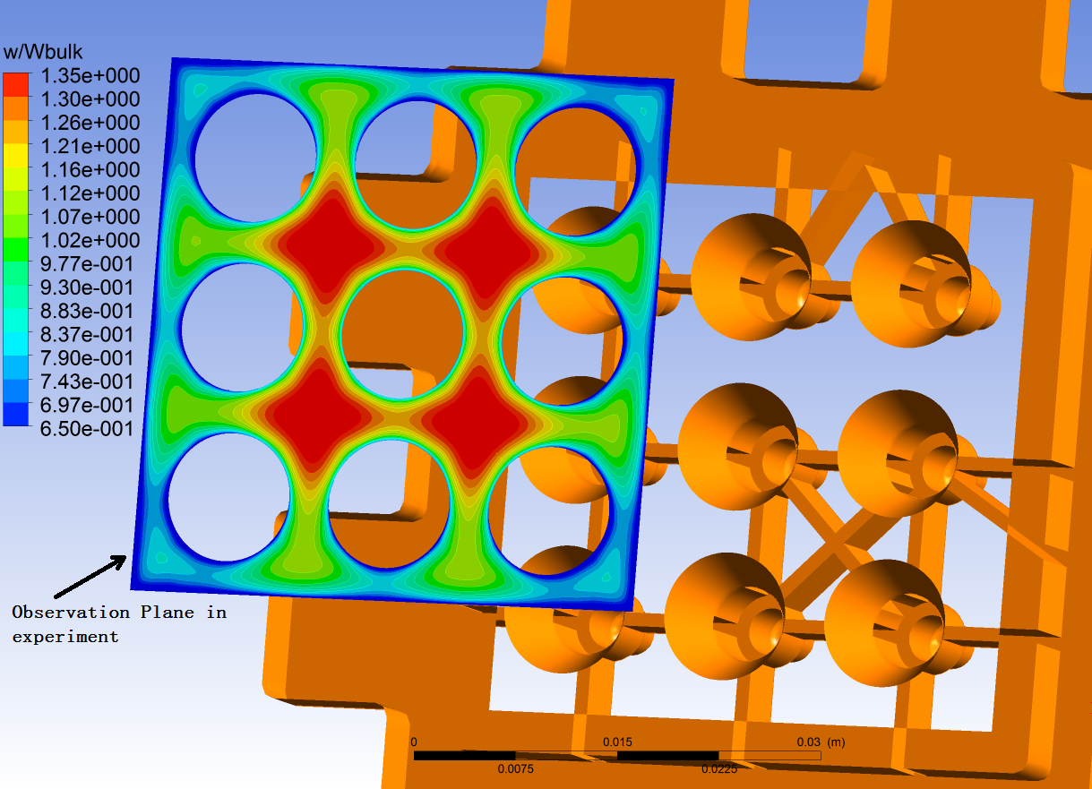
There is an observation plane, which is shown in Fig2, can be detected through measuring window. The plane, which locates 72mm above the outlet fixing device, is perpendicular to the measuring window. Through the window, axial velocity on the observation plane can be measured by LDV.
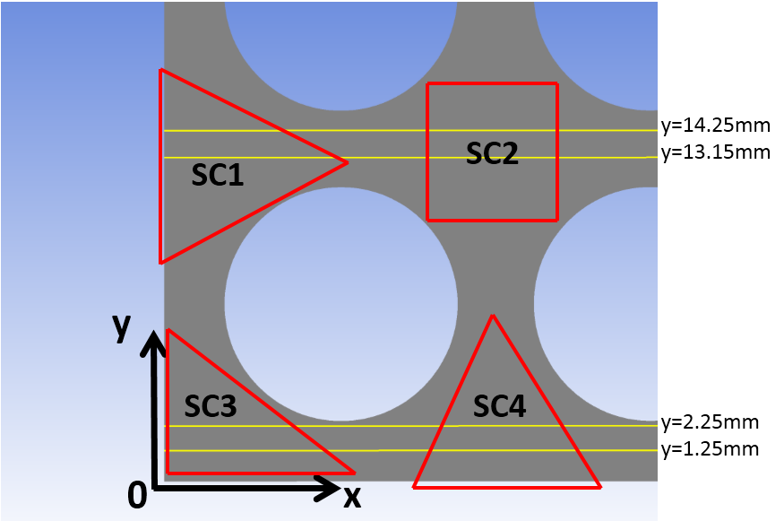
There are some observation lines on the observation plane. They are lines at y=1.25mm, 2.25mm and so on. The coordinate axis is shown in Fig3. Z axis is towards mainstream direction. The axial velocity profile on the observation lines can be obtained. And also there are some subchannels called SC1, SC2, SC3, SC4. They are shown in Fig3.
2. 2. Simulation methods
The flow investigated in this paper is isothermal. So the governing equations are mass and moment equation respectively [10]. The flow medium is water at 1atm.


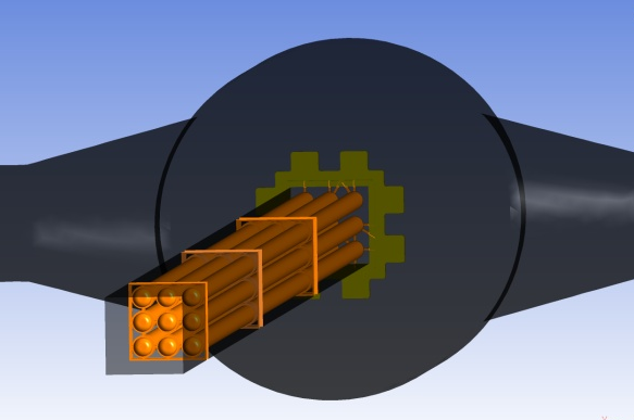
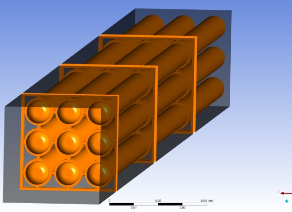
Two kinds of calculation domain were used in our simulation. The different calculation domains are shown in Fig4 and Fig5 respectively.
CFX was used to simulate the flowfield. ICEM was used to generate three kinds of mesh. They were coarse mesh, medium mesh and fine mesh. The three kinds of mesh's informations are shown in table1.
Table 1. Three kinds of grid.
| Mesh | Elements amount | Domain | Thickness of 1st layer |
| Coarse mesh | 3 437 863 | Same as Figure 4 | 0.5mm |
| Medium mesh | 5 077 233 | Same as Figure 4 | 0.2mm |
| Fine mesh | 19 404 362 | Same as Figure 5 | 0.03mm |
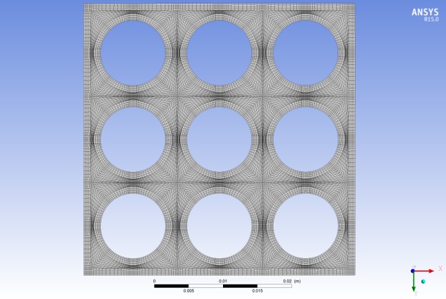
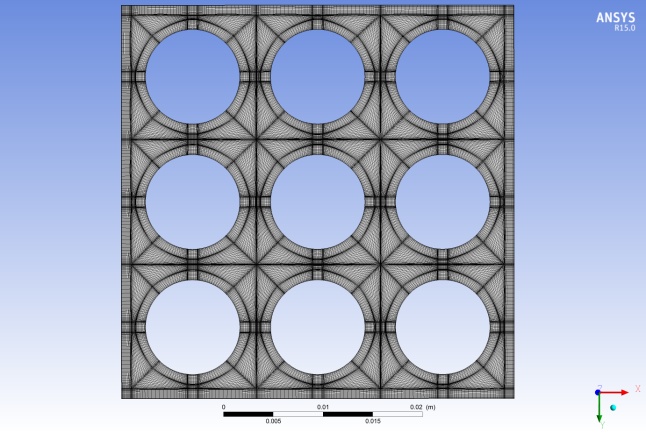
The difference between medium mesh and fine mesh on cross section is shown in Fig6 and Fig7. The three kinds of grid were used to investigate the mesh sensitive.The three kinds of grid were used to investigate the mesh sensitive. The results of coarse mesh are not as good as the other two kinds of mesh. So the results discussed below are the results from medium mesh and fine mesh.
The turbulence models used were BSL and LES WALE. BSL is one kind of RANS model. When the RANS model was used, the simulation was steady. While the LES was used, the simulation was transient. The time step is 1e-5s. The simulation condition was one of experiment condition at Re=15200.
When the BSL model was used, the results from fine mesh calculation had the best performance compared with experiment data. Because of our computing resource didn't satisfied the requirement of fine mesh LES calculation, we use medium mesh to simulate LES model.
3. RANS simulation results and experiment validation
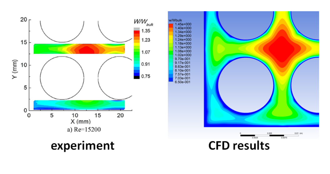
RANS turbulence model was used first, and the dimensionless axial velocity contour compared with experiment seemed to be almost the same. The experiment and simulation contour are shown in Fig8. [9]. The dimensionless axial velocity is defined as VD=w/W.
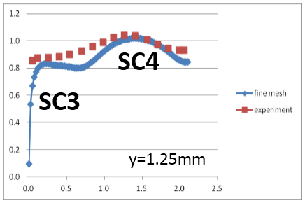
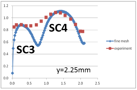
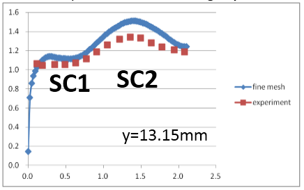
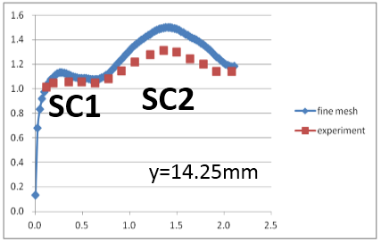
But when the quantitative comparison of dimensionless axial velocity on the observation lines was investigated, some obvious difference can be found, which is shown in Fig10. On line y=2.25mm axial velocity prediction of simulation was much smaller than experiment in domain between SC3 and SC4 shown in Fig10. And the problem in Fig9 is the same as Fig10. On line y=13.15mm and y=14.25mm axial velocity prediction of simulation was larger than experiment in subchannel SC2 shown in Fig11 and Fig12 respectively. The location of lines and subchannels mentioned above are shown in Fig3. The big difference between simulation results and experiment data in Fig9-12 would be induced by simulation models that were chosen. And RANS turbulence model is considered to be a major one.
4. LES simulation results and experiment validation
Peak values of dimensionless axial velocity on observation lines were not predicted well when the RANS turbulence model was used. So the LES turbulence was used to expect obtain better simulation data. Fig13-16 is the comparison between LES simulation results and experiment data.
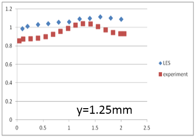
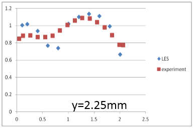
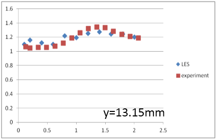
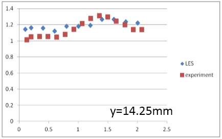
When the LES turbulence model was used, the peak value of axial velocity's prediction was much better than RANS turbulence model. But there were some deviation in the domain near experiment facility wall. This was caused by boundary layer not small enough. But when calculation resource was limited, we had to consider more efficient grid. And medium mesh was used to simulate LES turbulence model. So the axial velocity's prediction near wall was not as good as expected.
The fluctuation of axial velocity's contour based on LES transient simulation is shown in Fig17.b), compared with RANS steady simulation. The steady contour was different to transient contour obviously.
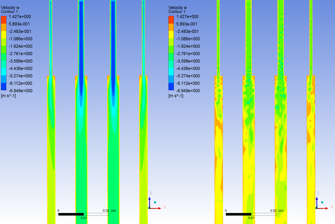
Figure 17. Axial velocity contour based on different turbulence model.
5. Conclusion
The experiment of 3x3 bundle flow for nuclear bundle design research was simulated by CFX. The performance of RANS and LES turbulence models for simulating flowfield around bundles were investigated. The calculation residual is under 10-3. And mesh sensitive was checked during RANS simulation. So the accuracy of the simulation is guaranteed. The simulation results were validated through comparing the experiment data.
The CFD contour results showed that reasonable results could be obtained by use of RANS turbulence model. But axial velocity peak value in some domain didn't have good agreement with experiment data.
The LES turbulence model was more accurate for predicting the axial velocity. But when the calculation resource is limited, more attention should be paid on the prediction results near walls, especially for the boundary layer grid.
Although simulation results was some sensitive to the turbulence model choice, both RANS and LES were highly recommended. Because reasonable results can be obtained no matter which model is chosen. RANS can be used for fast and efficient engineering simulation, while LES can be used for accurate research or design.
Acknowledgements
This work has been funded by the Chinese National Science and Technology Major Project under contract No. 2013ZX06004-008.
References
[1] B. S. Shin and S. H. Chang, "CHF experiment and CFD analysis in a 2 × 3 rod bundle with mixing vane," Nuclear Engineering and Design, vol. 239, no. 5, pp. 899-912, 2009. View Article
[2] S. Mimouni, F. Archambeau, M. Boucker, J. Lavieville and C. Morel, "A second order turbulence model based on a Reynolds stress approach for two-phase boiling flow and application to fuel assembly analysis," Nuclear Engineering and Design, vol. 240, no. 9, pp. 2225-2232, 2010. View Article
[3] L. Chandra and F. Roelofs, "CFD analyses of liquid metal flow in sub-channels for Gen IV reactors," Nuclear Engineering and Design, vol. 241, no. 11, pp. 4391-4403, 2011. View Article
[4] M. E. Conner, Y. A. Hassan and E. E. Dominguez-Ontiveros, "Hydraulic benchmark data for PWR mixing vane grid," Nuclear Engineering and Design, vol. 264, pp. 97-102, 2013. View Article
[5] B. L. Smith, "Assessment of CFD Codes for Nuclear Reactor Safety Problems NEA/SEN/SIN/AMA," 2005.
[6] T. Farkas and I. Tóth, "Fluent analysis of a ROSA cold leg stratification test," Nuclear Engineering and Design, vol. 240, no. 9, pp. 2169-2175, 2010. View Article
[7] M. E. Conner, E. Baglietto and A. M. Elmahdi, "CFD methodology and validation for single-phase flow in PWR fuel assemblies," Nuclear Engineering and Design, vol. 240, no. 9, pp. 2088-2095, 2010. View Article
[8] H. C. Rezende, A. A. Santos, M. A. Navarro and E. Jordão, "Verification and Validation of a thermal stratification experiment CFD simulation," Nuclear Engineering and Design, vol. 242, pp. 72-81, 2012. View Article
[9] J. Xiong, Y. Yu, N. Yu, X. Fu, H. Wang, X. Cheng and Y. Yang, "Laser Doppler measurement and CFD validation in 3 × 3 bundle flow," Nuclear Engineering and Design, vol. 270, pp. 396-403, 2014.View Article
[10] ANSYS Inc, "ANSYS Documentation Release 11.0ghg/default.asp?lang=En&n=040E378D-1".