Journal of Fluid Flow, Heat and Mass Transfer (JFFHMT)
ISSN: 2368-6111

Volume 3 - Year 2016 - Pages 25-33
DOI: 10.11159/jffhmt.2016.004
Boundary Control for an Arterial System
R.C. Cascaval1, C. D’Apice2, M.P. D’Arienzo2, R. Manzo2
1University of Colorado Colorado Springs, Department of Mathematics
1420 Austin Bluffs Pkwy, Colorado Springs, CO, United States 80918
radu@uccs.edu
2University of Salerno , Department of Computer Science
132 Via Giovanni Paolo II, Fisciano, SA, Italy 84084
cdapice@unisa.it; mdarienzo@unisa.it; rmanzo@unisa.it
Abstract - We consider a boundary control problem arising in the study of the dynamics of an arterial system which consists of one arterial segment (modeling the aorta in the cardiovascular system) coupled at the inflow with a pressurized chamber (modeling the left ventricle) via a valve. The opening and closing of the valve is dynamically determined by the pressure difference between the left ventricular and aortic pressures. Mathematically, this is described by a 1D system of coupled PDEs for the pressure and flow in the arterial segment, with a Dirichlet boundary condition imposed on the flow (when valve is closed) or on the pressure (when valve is open). At the outflow we impose a peripheral resistance model, which leads to a non-homogeneous Dirichlet condition. A numerical scheme based on the discontinuous Galerkin method is used to approximate the solution of the resulting system. We then use this methodology to simulate the heart rate variability observed in real physiological systems, by optimizing the timing of the heartbeat and the peripheral resistance, modeled using a terminal reflection coefficient, with the goal of achieving a prescribed mean pressure in the system.
Keywords: Boundary control, Aortic valve, Arterial pressure, Dispersion.
© Copyright 2016 Authors - This is an Open Access article published under the Creative Commons Attribution License terms Creative Commons Attribution License terms. Unrestricted use, distribution, and reproduction in any medium are permitted, provided the original work is properly cited.
Date Received: 2015-10-18
Date Accepted: 2016-01-26
Date Published: 2016-03-17
Nomenclature
In this paper, the following notations will be used:
A(x,t) |
cross-section area |
η(x,t) |
wall displacement |
r(x,t) |
radius of the artery |
u(x,t) |
average velocity |
P(x,t) |
hydrodynamic pressure |
Pext(t) |
external pressure |
PLV(t) |
left ventricular pressure |
Pref |
reference pressure |
Pavg |
mean pressure |
f(x,t) |
friction force |
β |
coefficient of elasticity |
h |
wall thickness |
μ |
blood viscosity |
ρ |
blood density |
ρω |
density of the wall |
E |
Young modulus |
HR |
heart rate |
τ |
duration of the systole |
Tpulse |
duration of a heart beat |
Wf |
forward characteristic wave |
Wb |
backward characteristic wave |
Rt |
reflection coefficient |
M |
length of the artery |
The values of the parameters used during the simulations are reported in section 4.
1. Introduction
The cardiovascular system transports oxygen and nutrients to all the tissues of the body, from where it removes carbon dioxide and other harmful waste products of cell metabolism. From a physical point of view, the system consists of a pump that propels a viscous liquid (the blood) through a network of flexible tubes. The heart provides energy to move blood through the circulatory system and is one key component in the complex control mechanism of maintaining pressure in the vascular system ([20]). The aorta is the main artery originating from the left ventricle and then bifurcates to other arteries, and is identified by several segments (ascending, thoracic, abdominal). There are several features of the aorta that have an effect on the blood flow, such as the tapering of the aorta or the fact that ascending aorta is arched (curved). Still, the functionality of the aorta, considered as a single segment, is worth exploring from a modeling perspective, in particular in relationship to the presence of the aortic valve.
There has been extensive literature describing the dynamics of the vascular network coupled with a heart model (e.g. [1], [7], [8], [9], [10], [16], [17]), the majority focusing on either a detailed description of the four chambers of the heart or on the spatial dynamics in the aorta, but not on both. In fact, there seem to be no studies addressing the heart rate variability based on the detailed spatial description of the pressure and flow patterns in the aorta. More broadly, theory and applications of optimization and control in spatial networks have been extensively developed in literature, and several numerical approaches have been successfully applied to telecommunications, transportation or supply networks ([5], [6], [15]).
In this paper we propose to capture through simulation and optimization the dynamics of the pressure and flow in the aorta as well as the heart rate variability. We take into account the elasticity of the aorta, considered as a single vessel, together with an aortic valve model at the inflow and a peripheral resistance model at the outflow (Section 2). We develop a numerical scheme to find approximate solutions to the system (Section 3) and then we describe and simulate a control mechanism for maintaining constant mean pressure in the aorta by allowing for variable heart rate and peripheral resistance (Section 4). Finally, we propose a spectral discretization of the optimal control problem to simulate this phenomenon (Section 5). The novelty of this paper is in considering the boundary control problem for a 1D PDE coupled with a valve model, which translates to a Dirichlet boundary condition for pressure during systole and for flow during diastole. The switch between the two type of boundary conditions is not prescribed a priori in time, but rather it is a function of the computed solution in time. This make the synthesis of the optimal control to be a non-standard problem, which is difficult to solve theoretically so we propose instead an effective numerical approach.
2. Mathematical Model
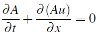
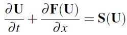
We start with the standard hyperbolic system (see [2], [14], [21]) which models cross-section area A(x,t) and average velocity u(x,t) in the spatial domain:
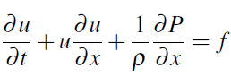
where f = f (x,t) is a friction force, usually taken to be
![]() , μ is the fluid viscosity, and P(x,t) is the
hydrodynamic pressure. Here we include the inertial effects
of the wall motion, described by the wall displacement
, μ is the fluid viscosity, and P(x,t) is the
hydrodynamic pressure. Here we include the inertial effects
of the wall motion, described by the wall displacement
![]() :
:
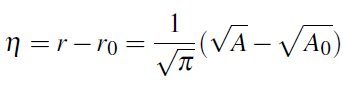
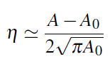
The fluid structure interaction is modeled using inertial forces, which gives the pressure law (see [3], [7])
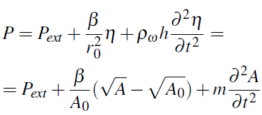
where r(x,t ) is the radius, r0(x,t); A0 = A(x0); Pext is
the external pressure, ![]() , σ is the Poisson ratio (usually
taken to be
, σ is the Poisson ratio (usually
taken to be ![]() , E is Young modulus, h is the wall
thickness,
, E is Young modulus, h is the wall
thickness, ![]() , ρω is the density of the wall.
The relation (4) was obtained by putting:
, ρω is the density of the wall.
The relation (4) was obtained by putting:
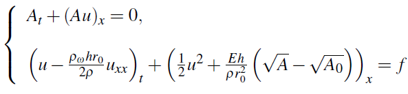
 This leads to the following Boussinesq system:
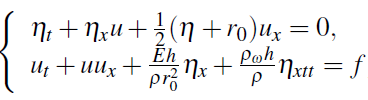
where ρ is the blood density. Considering the relation ![]() , we get the system:
, we get the system:
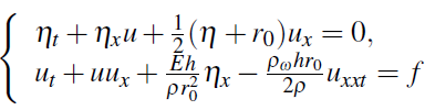
or, rearranging terms in u,
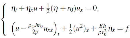
If we use cross-section area instead of the wall displacement, we have
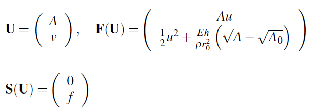
which can be written in compact form:
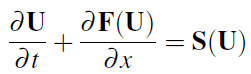
where
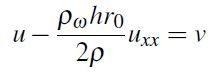
and ![]() is the solution of the boundary value problem
is the solution of the boundary value problem
together with boundary conditions that are indicated below.
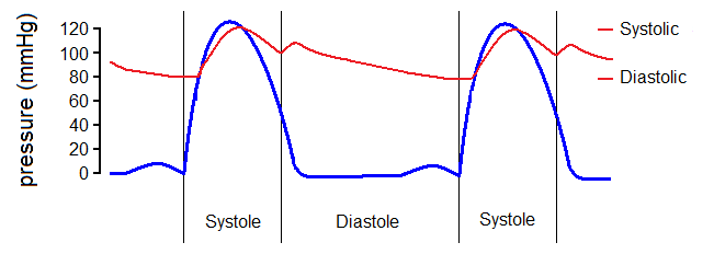
Inflow conditions (at x = 0) are implemented using a valve model, which mimics the real behavior of the physiological system. The aortic valve is one of the two semilunar valves of the heart and lies between the left ventricle and the aorta. It permits the flow of the blood from the left ventricle of the heart to the aorta. During ventricular systole, pressure rises in the left ventricle. When the pressure in the left ventricle rises above the pressure in the aorta, the aortic valve opens, allowing blood to exit the left ventricle into the aorta. When ventricular systole ends, pressure in the left ventricle rapidly drops. When the pressure in the left ventricle decreases below the aortic pressure, the aortic valve closes, and remains closed until the next heart beat. The opening and closing of valve is determined by the pressure difference between the left ventricle (PLV(t) ) and the aortic pressure. More specifically, the valve opens when
in which case the pressure at the inflow gets prescribed
and it closes when the velocity becomes negative, in which case the velocity at the inflow is prescribed to be zero:
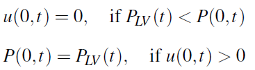
in which case the pressure at the inflow gets prescribed
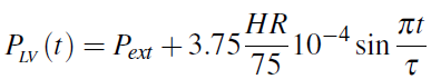
with HR representing the heart rate and t the duration of the systole, taken to be a quarter of the heart beat (τ = 15/HR). This model accounts for the fact that peak amplitude of the left ventricular pressure depends on the heart rate.
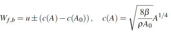
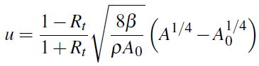
As terminal condition, we have used a model with terminal reflection coefficient Rt, (see [2]), which is based on the assumption that Wb is proportional to Wf:
where ![]() Here Wb is the backward characteristic
and Wf is the forward characteristic of the hyperbolic system
(9):
Here Wb is the backward characteristic
and Wf is the forward characteristic of the hyperbolic system
(9):
Note that Rt = 1 corresponds to u = 0, which means the outflow
is completely blocked, while Rt = -1 corresponds to A = A0. For general values of ![]() the boundary conditions is
the boundary conditions is
This is a nonlinear relation between the two components (area and velocity) of the system of PDEs.
We note that the reduced 1D model (1)–(2) can be derived ([21]) from the full 3D fluid flow equations under both the assumption of newtonian or non-newtonian nature for the fluid, the difference being in the nonlinearity of the velocity. Here we followed the standard non-newtonian assumption of a blunt velocity profile across the vessel wall, which is typical for blood flow in large arteries. Alternative (and more realistic) models for the rheology of the blood (such as Casson model, [18], [23], which assumes a nonlinear stress strain relation for the fluid) will lead to different expressions for the friction forces in the reduced model and to different nonlinear terms for the momentum equation. While these models are worth considering for a more realistic mathematical model (see also comments in the conclusion section), for the scope of the present paper it is sufficient to stay with simplest model for the fluid and fluid structure interactions, since we do not expect significantly different qualitative conclusions if we were to incorporate other models.
3. Numerical Discretization
In order to solve the system (9)–(11) on Ω = [0;L] we use a discontinuous Galerkin scheme for the first equation and a spectral method for the second one.
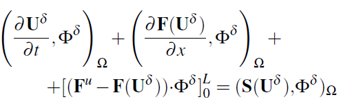
We write the weak formulation of the problem, approximate
U(x,t) with its discretized expansion ![]() and integrate
twice by part (for details see [21]), so we get:
and integrate
twice by part (for details see [21]), so we get:
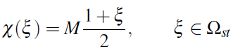
To simplify the method, we have mapped each elemental region
onto the standard element ![]() .
This mapping is defined as
.
This mapping is defined as
and its inverse is given by
We selected as expansion basis the Legendre polynomials
![]() , with k the polynomial order, because they are orthogonal
with respect to the product inner product of L2. In this
way, the solution is expanded on Ω as
, with k the polynomial order, because they are orthogonal
with respect to the product inner product of L2. In this
way, the solution is expanded on Ω as
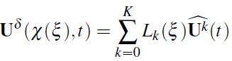
with ![]() the time-varying coefficients of the expansion.
We have chosen Legendre points (which are the zeros of Legendre
polynomials) as collocation points.
Replacing (13) in (12) and letting
the time-varying coefficients of the expansion.
We have chosen Legendre points (which are the zeros of Legendre
polynomials) as collocation points.
Replacing (13) in (12) and letting ![]() , we obtain the
following system of 2(K + 1) differential equations to be solved:
, we obtain the
following system of 2(K + 1) differential equations to be solved:
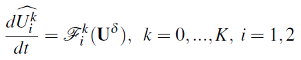
where ![]() , are each of the two components of
, are each of the two components of ![]() and
and

with M as the length of the edge. The method is completed with a second-order Adams-Bashforth timeintegration scheme:
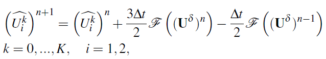
in which ![]() is the time step and n the number of every time
step. To calculate the integrals we use a Gauss quadrature
formula of order
is the time step and n the number of every time
step. To calculate the integrals we use a Gauss quadrature
formula of order ![]()
The upwinded fluxes ![]() are computed solving a Riemann
problem that takes into account the characteristic information
moving away. At a time t, each interface separates
two constant states,
are computed solving a Riemann
problem that takes into account the characteristic information
moving away. At a time t, each interface separates
two constant states, ![]() and
and ![]() , and we need to
determine the two upwinded states,
, and we need to
determine the two upwinded states, ![]() and (
and (![]() ,
originated on each side of interface at time
,
originated on each side of interface at time ![]() . To do this, the following equations are required:
. To do this, the following equations are required:
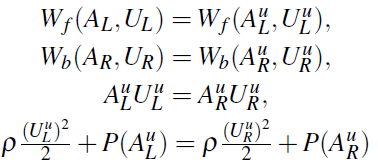
The first two equations come from the assumption that the flow between two initial states is inviscid, and the forward characteristic information, Wf , and the backward characteristic information,Wb:
To approximate the second order derivative of u, we
use the spectral method involving Chebyshev differentiation
matrixes, defined for the Chebyshev collocation points
![]() as follows (see [22]):
as follows (see [22]):
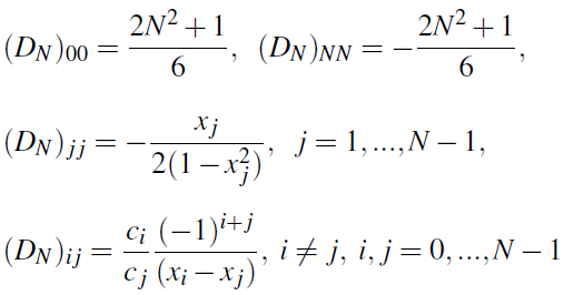
where
This discretization can be coupled with the discontinuous Galerkin scheme described above, by matching the solution at Chebyshev points, performing the derivative using these points, then returning back to the Legendre points.
Using this method, we compare dispersion (ρω > 0) and dispersionless (ρω = 0) models. We choose a rather high density for the wall in order to underline the difference. The result of the simulation is given below:
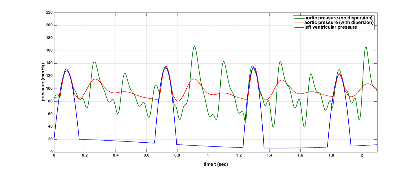
We observe that for the dispersionless case, the multiple peaks between heartbeats indicate that the waves which originate during a systole reflect off the boundaries and travel back and forth (with decreased amplitudes) during the diastole. These can be used to compute the speeds of the pulse waves in relation to the heart rates, similar to [12].
In the dispersive case, the pressure waves have much
fewer oscillations than in the dispersionless case. This can
be explained by the higher density of the wall, hence higher
wall inertia, and consequently fewer transversal oscillations.
Since these are temporal recordings at one spatial location,
these show an averaging effect due to dispersion of flow
along the vessel, and not a dampening of the waves. In simulations
we also witnessed a greater degree of the averaging
when the wall density increase. If on the other hand we keep
all the parameters (e.g. wall density etc) but we consider a
shorter length of the vessel M, then by rescaling the spatial
variable ![]() , one obtains a similar effect - of increasing
the value of the wall density, and hence of averaging the
pressure pulses originating from the left ventricle. Another
effect which can be captured in our numerical model is the
variable (along the vessel length) radii and elasticity.
, one obtains a similar effect - of increasing
the value of the wall density, and hence of averaging the
pressure pulses originating from the left ventricle. Another
effect which can be captured in our numerical model is the
variable (along the vessel length) radii and elasticity.
4. Optimization of Mean Arterial Pressure
We now use the numerical model developed so far to perform several optimization tasks, in the same spirit as [4]. The first one is to maintain the mean arterial pressure close to a prescribed reference value (Pref), in presence of external pressure changes. The external pressure Pext is taken to vary with time, to mimic the respiratory cycle, according to
Here we consider an arterial segment of length 0.5 m. The following parameter values are used throughout the sequel: μ= 3 x 10⁻¹⁰ mmHg (viscosity of the blood), ρ = 1050 Kg/m3 (blood density), β = 1418 N/m (elasticity parameter), Pref = 100 mmHg and the total time of the simulation is tfinal = 10 sec.
We are interested in finding the optimal HR (and later also terminal resistance Rt - assumed constant during one heartbeat) which leads to the minimization of the following cost functional
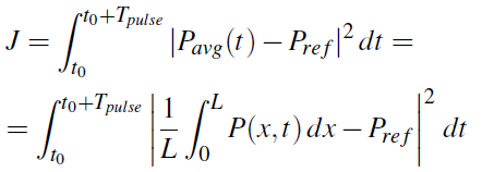
Here the integration is done using an entire heartbeat, with duration Tpulse = 60/HR. The systolic period is taken to be consistently one quarter of Tpulse.
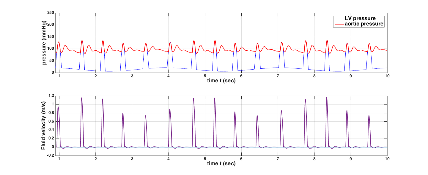
Upon optimization on HR alone, we obtain the following 10-sec recording of the aortic pressure, plotted together with the left ventricular pressure. The first heartbeat has not been included in the plot, since the initial condition is anomalous and does not affect the subsequent dynamics.
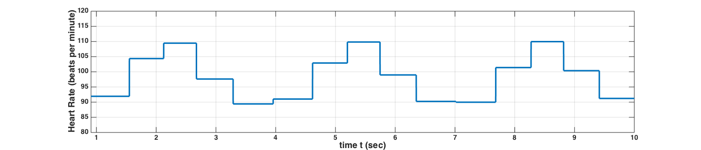
When including the terminal resistance as one of the optimization parameters, we notice a different pattern of the optimal HR, which is to be expected. The variability of the HR and terminal resistance Rt are shown in the figures below:
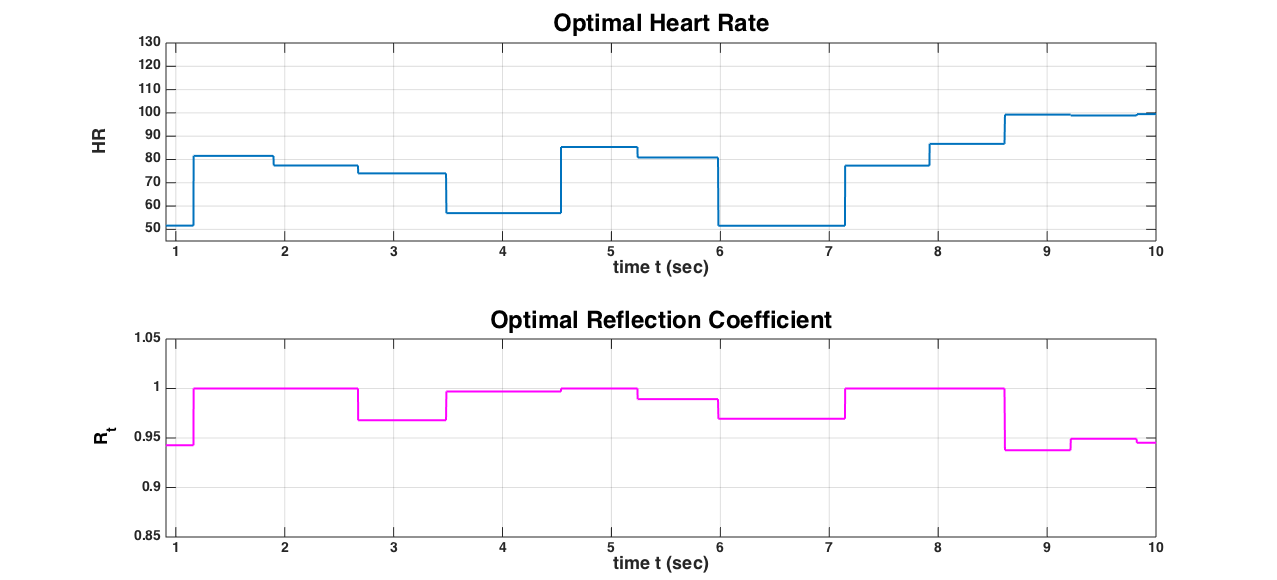
We observe that the terminal resistance Rt is close to 1, which means that there is almost a complete reflection of the characteristic waves and almost complete blockage in the terminal site. HR varies in sync with the respiratory cycle, but the presence of peripheral resistance mechanism is breaking the periodicity of the HR variability, which is what is observed in the real system. Also we note that comparing this range of HR with the results above (when only HR was used in optimization, keeping Rt = 0.9 fixed), leads us to the conclusion that in order to maintain a prescribed mean pressure over one heart beat increasing the Rt (even to its maximal value) is more efficient than increasing the HR. Naturally, the consideration of a single arterial segment (aorta) avoids the effects of the complexity of the vascular network, which would add additional irregular behavior in the HR variability.
5. Optimal Control of Mean Arterial Pressure
We consider the optimal control problem of achieving a prescribed mean arterial pressure by allowing for variable terminal resistance Rt = R during the time period [t0, t0 + Tpulse] of one heart beat, Tpulse = 60/HR. Note that we do not perform optimization on the heart rate HR, since the HR can be controlled separately.
For simplicity, we formulate our optimal control problem using the dispersionless system:
where
with domain
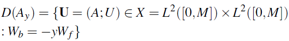
encodes the boundary conditions in terms of the control variable y (expressed as boundary control). In our application y = Rt is the terminal reflection coefficient which is allowed to vary during the time period of one heart beat T = 60/HR.
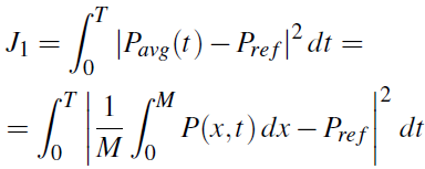
The optimization task is defined as follows: determine the optimal terminal resistance that achieves the desired mean pressure. This is a nontrivial fact, since we assume the external pressure is variable (possibly due to a sudden drop or rise in pressure,) the system tries to find the optimal value of the Heart Rate that achieves the desired goal.
The optimal control problem is to find y = y(t) that minimizes the integral
Due to the non-standard nature of the Dirichlet boundary control problem posed, we expect that the full PDE boundary control will lead to an adjoint formulation of the optimal control problem involving integral formulation of the necessary condition for optimality (see [13]). This will be pursued elsewhere. In the sequel we turn to a pseudo spectral discretization of the optimal control problem [15], [19]. The discretization uses the same framework as the numerical scheme already discussed, using Legendre polynomials and Legendre Gauss nodes. For simplicity, we describe this discretization procedure on an optimal control problem for the Dirichlet boundary control for the viscous Burgers equation:
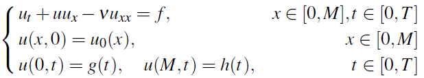
with g and h the controls, and cost functional to be minimized
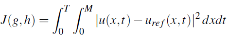
where uref is a reference (desired) profile for the solution.
We choose the Legendre-Gauss-Lobatto (LGL) points
![]() , (cf. [19]), where
x1,...xN-1are the zeros of L'N, the derivatives of the Legendre
polynomial of degree N and we approximate the function
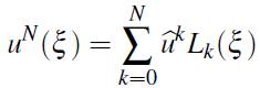
u using the Lagrange interpolant for the points (xj,u(xj)).
Then we introduce the approximate solution:
, (cf. [19]), where
x1,...xN-1are the zeros of L'N, the derivatives of the Legendre
polynomial of degree N and we approximate the function
u using the Lagrange interpolant for the points (xj,u(xj)).
Then we introduce the approximate solution:
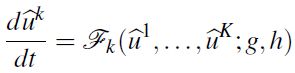
and convert the optimal PDE control problem to the optimal ODE control problem:
Minimize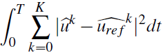
subject to
Here the right-hand side is obtained from the variational formulation of the PDE:
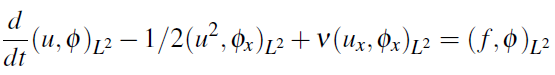
If we restrict the test functions to polynomials of degree N or less, then we obtain
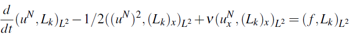
or
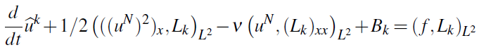
Here the boundary contribution is
This leads to the expression for the right hand side in (16):
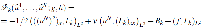 .
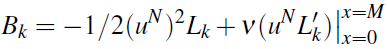
.Note that Bk can be written in terms of the boundary control as:
 .
.Applying Pontryagin minimum principle we are led to an adjoint problem for the adjoint variables λk, k = 0,...K.
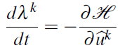
where
is the Hamiltonian. A necessary optimal condition is then
A similar construction can be carried out for the inviscid Euler system (15), which yields, upon discretization using the same Gauss Legendre Lobatto points, the system
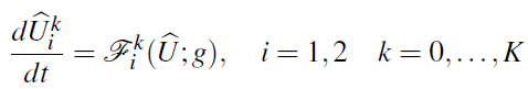
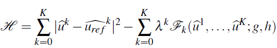
The adjoint system takes the form
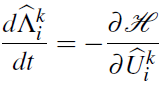
where the Hamiltonian function is
Applying of the Pontryagin minimum principle leads to the
computation of the optimal ![]() . We remark that while
this is a nonstandard application of the Pontryagin minimum
principle, it follows the same steps as the traditional principle
where pure Dirichlet boundary conditions are involved.
A numerical implementation of this discretized control problem
as well as a more detailed discussion on the connection
with the full PDE boundary control will be reported elsewhere.
. We remark that while
this is a nonstandard application of the Pontryagin minimum
principle, it follows the same steps as the traditional principle
where pure Dirichlet boundary conditions are involved.
A numerical implementation of this discretized control problem
as well as a more detailed discussion on the connection
with the full PDE boundary control will be reported elsewhere.
6. Conclusions
The numerical optimization results presented here are relevant for understanding how boundary control affects the dynamics of the pressure and flow in an arterial segment, via the valve model at the root of the vascular network and via peripheral resistance model at the outflow. The consideration of a single edge can be viewed as certainly restrictive from a physiological point of view, but can help in further studies where the entire vascular network is considered. Furthermore, more realistic models for the rheology of blood, for the mechanical characteristics of the tube walls and for the fluid-structure interactions are worthy to be incorporated in the optimization studies presented here, something we intend to report elsewhere.
Acknowledgement
R.C. was supported by a grant from the UCCS BioFrontiers Center of the University of Colorado. R.C. is also grateful for the hospitality of the Universit`a degli Studi di Salerno during his stay there.
References
[1] J. A. Arimon, K. H. Parker, J. Peiró and S. J. Sherwin, "Analysing the pattern of pulse waves in arterial networks: a time-domain study," Journal of Engineering Mathematics, vol. 64, no. 4, pp. 331-351, 2009. View Article
[2] J. A. Arimon, "Numerical modelling of pulse wave propagation in the cardiovascular system: development, validation and clinical applications," Imperial College London, London, 2006. View Article
[3] R. C. Cascaval, "A Boussinesq model for pressure and flow velocity waves in arterial segments," Mathematics and Computers in Simulation, vol. 82, no. 6, pp. 1047-1055, 2012. View Article
[4] R. C. Cascaval, C. DApice, M. DArienzo and R. Manzo, "Flow optimization in vascular networks," Mathematical Biosciences and Engineering, vol. 262, 2015. View Article
[5] C. D'Apice, R. Manzo and . B. Piccoli, "A Fluid Dynamic Model for Telecommunication Networks with Sources and Destinations," SIAM Journal on Applied Mathematics, vol. 68, no. 4, pp. 981-1003, 2008. View Article
[6] C. DApice, R. Manzo and B. Piccoli, "Modelling supply networks with partial differential equations," Quarterly of Applied Mathematics, vol. 67, no. 3, pp. 419-440, 2009. View Article
[7] L. Formaggia, D. Lamponi and A. Quarteroni, "Onedimensional models for blood flow in arteries," Journal of Engineering Mathematics, vol. 47, no. 3, pp. 251-276, 2003. View Article
[8] L. Formaggia, D. Lamponi, M. Tuveri and A. Veneziani, "Numerical modeling of 1D arterial networks coupled with a lumped parameters description of the heart," Computer Methods in Biomechanics and Biomedical Engineering, vol. 9, no. 5, pp. 273-288, 2006. View Article
[9] L. Formaggia, A. Quarteroni and A. Veneziani, Cardiovascular Mathematics: Modeling and simulation of the circulatory system, Springer Verlag, 2010. View Article
[10] F. Hoppensteadt and C. Peskin, Modeling and Simulation in Medicine and the Life Sciences, New York: Springer science and business media, 2004. View Article
[11] J. M. Lellouche, J. L. Devenon and I. Dekeyser, "Boundary control of Burgers' equationa numerical approach," Computers and Mathematics with Applications, vol. 28, no. 5, pp. 33-44, 1994. View Article
[12] J. S. Lillie, "Pulse Wave Velocity Prediction and Compliance Assessment in Elastic Arterial Segments," Cardiovascular Engineering and Technology, vol. 6, no. 1, pp. 49-58, 2015. View Article
[13] B. S. Mordukhovich, Variational Analysis and Generalized Differentiation I: Basic Theory, New York: Springer Heidelberg, 2006. View Article
[14] A. S. Liberson, J. S. Lillie and D. A. Borkholder, "Numerical Solution for the Boussinesq Type Models with Application to Arterial Flow," Journal of Fluid Flow, Heat and Mass Transfer, vol. 1, pp. 9-15, 2014. View Article
[15] A. Noack and A.Walther, "Adjoint concepts for the optimal control of Burgers equation," Computational Optimization and Applications, vol. 36, no. 1, pp. 109-133, 2007. View Article
[16] J. T. Ottesen, M. S. Olufsen and J. K. Larsen, "Applied Mathematical Models in Human Physiology," Society for Industrial and Applied Mathematics, 2004. View Article
[17] P. Reymond, F. Merenda, F. Perren and N. Stergiopulos, "Validation of a One-Dimensional Model of the Systemic Arterial Tree," The American Journal of Physiology - Heart and Circulatory Physiology, vol. 297, no. 1, pp. 208-222, 2009. View Article
[18] A. M. Robertson, A. Sequeira and R. G. Owens, "Rheological models for blood," Cardiovascular Mathematics, Milano, Springer-Verlag, 2009, pp. 211-241. View Article
[19] I. M. Ross and M. Karpenko, "A review of pseudospectral optimal control: From theory to flight," Annual Reviews in Control, vol. 36, no. 2, pp. 182-197, 2012. View Article
[20] L. Rowell, Human Cardiovascular Control, New York: Oxford University Press, 1993. View Article
[21] S. J. Sherwin, L. Formaggia, J. Peir and V. Franke, "Computational modelling of 1D blood flow with variable mechanical properties and its application to the simulation of wave propagation in the human arterial system," International Journal for Numerical Methods in Fluids, vol. 43, no. 6-7, pp. 673-700, 2003. View Article
[22] L. N. Trefethen, "Spectral Methods in Matlab," Society for Industrial and Applied Mathematics, 2000. View Article
[23] J. Venkatesan, D. S. Sankar, K. Hemalatha and Y. Yatim, "Mathematical Analysis of Casson Fluid Model for Blood Rheology in Stenosed Narrow Arteries," Journal of Applied Mathematics, vol. 2013, pp. 1-11, 2013. View Article